Technology scout

Now it’s time for my favourite graph visualization framework. As an introduction I cite from the Cytoscape website:

Cytoscape is an open source software platform for visualizing molecular interaction networks and biological pathways and integrating these networks with annotations, gene expression profiles and other state data.

Cytoscape.js as a side project is a JavaScript library designed to build graph theory related data evaluation and visualization applications on the web. It comes with some layout renderers but is open to other visualization libraries such as Cola.js. Cola is a constraint based layout library with some very interesting features. In this context, we will use it only as a layout engine for the graph.

How does it look?

When playing around with this graph you will probably notice two things:

1. When dragging around a single node all the other nodes of the graph remain calm and don’t wiggle around like in most physical based layouts.
2. When reloading this page you will always see the same arrangement of nodes. The graph is stable to reloads.

These two feature result from the way Cola.js renders the graph and are very useful for real world applications. While it’s big fun wobbling and dragging around nodes in a real application you would always like to see the same graph when reloading the same data. And manipulating the arrangement should not affect nodes not touched. The complete source code can be found in the GitHub repository.

How does it work?

Once again we start by including the stuff needed. And this are the two libraries and an adaptor to use Cola.js from within Cytoscape.js:

<script src="/graphs/common/cola.js"></script>
<script src="/graphs/common/cytoscape.js"></script>
<script src="/graphs/common/cytoscape-cola.js"></script>

The adaptor can also be found on GitHub.

The HTML body contains a div to render the graph into:

<div id="cy"></div>

The remainder of the index.html file consists of a script:

var elems = [
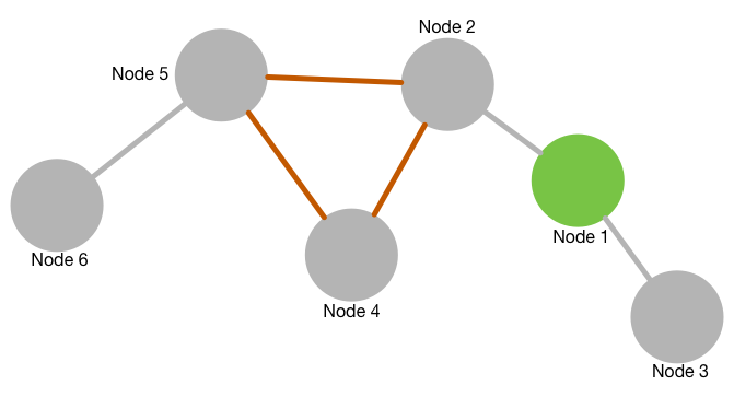
    {data: {id: '1', name: 'Node 1', nodecolor: '#88cc88'}},
    {data: {id: '2', name: 'Node 2', nodecolor: '#888888'}},
    {data: {id: '3', name: 'Node 3', nodecolor: '#888888'}},
    {data: {id: '4', name: 'Node 4', nodecolor: '#888888'}},
    {data: {id: '5', name: 'Node 5', nodecolor: '#888888'}},
    {data: {id: '6', name: 'Node 6', nodecolor: '#888888'}},
    {
        data: {
            id: '12',
            source: '1',
            target: '2',
            linkcolor: '#888888'
        },
    },
    {
        data: {
            id: '13',
            source: '1',
            target: '3',
            linkcolor: '#888888'
        },
    },
    {
        data: {
            id: '24',
            source: '2',
            target: '4',
            linkcolor: '#ff8888'
        },
    },
    {
        data: {
            id: '25',
            source: '2',
            target: '5',
            linkcolor: '#ff8888'
        },
    },
    {
        data: {
            id: '45',
            source: '4',
            target: '5',
            linkcolor: '#ff8888'
        }
    },
    {
        data: {
            id: '46',
            source: '4',
            target: '6',
            linkcolor: '#888888'
        }
    }];
var cy = cytoscape({
    container: document.getElementById('cy'),
    elements: elems,
    style: cytoscape.stylesheet()
            .selector('node').style({
                'background-color': 'data(nodecolor)',
                label: 'data(name)',
                width: 25,
                height: 25
            })
            .selector('edge').style({
                'line-color': 'data(linkcolor)',
                width: 3
            })
});
cy.layout({name: 'cola', padding: 10});

Lines 2 to 7 define the nodes with their name/caption and colour. Lines 8 to 54 define the edges in a similar way. Lines 56 to 70 define the Cytoscape container and attach dynamic properties to the nodes and edges. Line 71 finally kicks off the layout rendering. Note: up to that last line we specified exactly no rendering or geometry information! By changing the name of the renderer from cola  to one of the built-ins (circle  or cose  are fun to play with!) you can get a completely different outout.

As a last remark I strongly recommend to have a look at the graph theoretical and practical routines and algorithms the Cytoscape.js library has to offer.

Arbor.js is written by Christian Swineheart from Samizdat Drafting Co. The documentation is concise even though the main page navigation as animated tree layout always drives me crazy :) The example I present here only depends on arbor.js and jQuery. Graph definition is for shortness and clarity done by calls to addNode  and addEdge  methods of the ParticleSystem renderer.

How does it look?

As you can see, the physical simulation is much more fluid and undamped than with Alchemy.js. I’m pretty much shure this can be changed to some degree with a different initialization of the particle system as described in the reference documentation. Once again, the complete source code, in this case consisting only of an index.html file, can be found in the GitHub repository.

How does it work?

Once again in the header we start by loading the stuff needed:

<script src="/graphs/common/jquery-2.1.3.js"></script>
<script src="/graphs/common/arbor.js"></script>
<script src="/graphs/common/arbor-tween.js"></script>

arbor-tween.js is not really needed for this example as it allows gradual transitions in the data object of nodes and edges. Arbor.js by default renders its graph in a HTML5 canvas, in the body we need to define this:

<canvas id="viewport" width="800" height="500"></canvas>

The remainder of the file consists of a function defining and binding the renderer object to the canvas and constructing the graph:

(function ($) {
        var Renderer = function (canvas) {
                var canvas = $(canvas).get(0);
                var ctx = canvas.getContext("2d");
                var particleSystem;
                var that = {
                        init: function (system) {
                                particleSystem = system;
                                particleSystem.screenSize(canvas.width, canvas.height);
                                particleSystem.screenPadding(100);
                                that.initMouseHandling()
                        },
                        redraw: function () {
                                ctx.fillStyle = "white";
                                ctx.fillRect(0, 0, canvas.width, canvas.height);
                                particleSystem.eachEdge(function (edge, pt1, pt2) {
                                        ctx.strokeStyle = edge.data.linkcolor;
                                        ctx.lineWidth = 3;
                                        ctx.beginPath();
                                        ctx.moveTo(pt1.x, pt1.y);
                                        ctx.lineTo(pt2.x, pt2.y);
                                        ctx.stroke();
                                });
                                particleSystem.eachNode(function (node, pt) {
                                        ctx.beginPath();
                                        ctx.arc(pt.x, pt.y, 15, 0, 2 * Math.PI);
                                        ctx.fillStyle = node.data.nodecolor;
                                        ctx.fill();
                                        ctx.font = "18px Arial";
                                        ctx.fillStyle = "#000000";
                                        ctx.fillText(node.data.name, pt.x + 20, pt.y + 5);
                                });
                        },
                        initMouseHandling: function () {
                                var dragged = null;
                                var handler = {
                                        clicked: function (e) {
                                                var pos = $(canvas).offset();
                                                _mouseP = arbor.Point(e.pageX - pos.left, e.pageY - pos.top);
                                                dragged = particleSystem.nearest(_mouseP);
                                                if (dragged && dragged.node !== null) {
                                                        dragged.node.fixed = true;
                                                }
                                                $(canvas).bind('mousemove', handler.dragged);
                                                $(window).bind('mouseup', handler.dropped);
                                                return false;
                                        },
                                        dragged: function (e) {
                                                var pos = $(canvas).offset();
                                                var s = arbor.Point(e.pageX - pos.left, e.pageY - pos.top);
                                                if (dragged && dragged.node !== null) {
                                                        var p = particleSystem.fromScreen(s);
                                                        dragged.node.p = p
                                                }
                                                return false;
                                        },
                                        dropped: function (e) {
                                                if (dragged === null || dragged.node === undefined) return;
                                                if (dragged.node !== null) dragged.node.fixed = false;
                                                dragged.node.tempMass = 1000;
                                                dragged = null;
                                                $(canvas).unbind('mousemove', handler.dragged);
                                                $(window).unbind('mouseup', handler.dropped);
                                                _mouseP = null;
                                                return false;
                                        }
                                };
                                $(canvas).mousedown(handler.clicked);
                        }
                }
                return that;
        }
        $(document).ready(function () {
                var sys = arbor.ParticleSystem(700, 700, 0.5);
                sys.renderer = Renderer("#viewport");
                sys.addNode('Node 1', {name: "Node 1", nodecolor: "#88cc88"});
                sys.addNode('Node 2', {name: "Node 2", nodecolor: "#888888"});
                sys.addNode('Node 3', {name: "Node 3", nodecolor: "#888888"});
                sys.addNode('Node 4', {name: "Node 4", nodecolor: "#888888"});
                sys.addNode('Node 5', {name: "Node 5", nodecolor: "#888888"});
                sys.addNode('Node 6', {name: "Node 6", nodecolor: "#888888"});
                sys.addEdge('Node 1', 'Node 3', {linkcolor: "#888888"});
                sys.addEdge('Node 1', 'Node 2', {linkcolor: "#888888"});
                sys.addEdge('Node 2', 'Node 5', {linkcolor: "#ff8888"});
                sys.addEdge('Node 2', 'Node 4', {linkcolor: "#ff8888"});
                sys.addEdge('Node 4', 'Node 5', {linkcolor: "#ff8888"});
                sys.addEdge('Node 5', 'Node 6', {linkcolor: "#888888"});
        })
})(this.jQuery);

Lines 2 to 73 define the Renderer, in detail:

• get the HTML5 canvas (line 3)
• grab its 2D context (line 4)
• an init function for the particle system (lines 7 to 12)
• a redraw function actually drawing the graph (lines 13 to 33) by iterating over all nodes and edges
• defining a pretty basic mouse handling (lines 34 to 69)

In line 75 we get a particle system, set the rendering to the canvas in line 76 and define nodes (lines 76 to 81) and edges (lines 82 to 87). That’s pretty much all.

Alchemy.js is a library developed by graphAlchemist (site defunct). The documentation could be better and more detailed but it works. Like many other libraries it leverages other libraries to do “the basic stuff”. In this case it is it depends on:

• jQuery
• D3
• lodash

Alchemy uses GraphJSON (similar to GeoJSON) as input format, which is quite nice but undocumented since the website graphjson.io doesn’t exist any more. Looks as if support for it ceded with the graphAlchemist web site …

How does it look?

Like all demos I’ll show it’s a fully functional mini demo, so you can drag the nodes around. I’ll present excerpts of the code to explain. The complete code can be found in a GitHub repository.

How does it work?

Our example consists of an index.html file, a GraphJSON data file and the library stuff. In the index.html we first load the stuff needed:

<link rel="stylesheet" href="/graphs/common/alchemy/alchemy.css"/>
<script src="/graphs/common/jquery-2.1.3.js"></script>
<script src="/graphs/common/d3.js"></script>
<script src="/graphs/common/lodash.js"></script>

The body contains a div to put the graph in and the include for the base library itself:

<div class="alchemy" id="alchemy"></div>
<script src="/graphs/common/alchemy/alchemy.js"></script>

Finally there’s the code producing the graph:

var config = {
    dataSource: '/graphs/alchemy/data/network.json',
    graphWidth: function() {return 800},
    graphHeight: function() {return 500},
    backgroundColor: "#ffffff",
    nodeCaptionsOnByDefault: true,
    caption: function(node){
        return node.caption;
    },
    nodeTypes: {
        "role": ["greyone", "greenone"]
    },
    edgeTypes: {
        "caption": ["greyone", "redone"]
    },
    nodeStyle: {
        "greyone": {
            color: "#888888",
            borderWidth: 0,
            radius: 15
        },
        "greenone": {
            color: "#88cc88",
            borderWidth: 0,
            radius: 15
        }
    },
    edgeStyle: {
        "greyone": {
            color: "#888888",
            width: 3
        },
        "redone": {
            color: "#ff8888",
            width: 3
        }
    }
};
alchemy = new Alchemy(config)

As you can see, nearly everything is done in a configuration object. Line 2 defines the source of the GraphJSON file, lines 3 & 4 set the dimensions of the SVG element. The setting of nodeCaptionsOnByDefault  in line 6 switches on the display of the node titles. Otherwise they would only show up when hovering with the mouse. Lines 7 to 9 define a callback function defining what to display as a caption / title. Lines 10 to 15 define valid values for grouping edges and nodes. Nodes are grouped by the role attribute, edges by caption. Lines 16 to 37 define how these groups of edges and nodes should be formatted. There are other, more direct ways to style a graph in Alchemy.js but I wanted to show the (for me) most elegant way. Finally line 39 kicks off the rendering of the graph with the given configuration.

This post starts a small series of articles, that will present some JavaScript graph plotting libraries and show how to draw more or less the same simple demo graph with these different libs.

What is a graph?

Graph theory is a mathematical discipline that studies networks of nodes and links or edges connecting them. Graphs are useful for many applications: social media networks, streets connecting cities, transfers connecting bank accounts or networks of people, addresses, bank accounts and cars connected via insurance claims and events. We’ll deal with some of those applications later on when discussing the application of network and graph paradigms to visualizing fraudulent actions.

Which libraries have I examined?

The internet is full, I mean literally FULL of libraries to display networked graphs. I had to choose some and discard others. First I decided to neglect commercial libraries that don’t have an open source edition. Then I stopped evaluating libs when I recognized that the documentation is too poor or functionality too limited to further investigate. So here is the list in alphabetical order:

• Alchemy.js
• Arbor.js
• Cytoscape with Cola.js rendering
• D3.js
• D3.js with Cola.js rendering
• Infovis Toolkit
• vis.js

Libraries I didn’t evaluate due to licensing constraints:

• Keylines
• yFiles for HTML

Libraries I gave up on:

• Dracula Graph Library (Graph Dracula … you understand … haha)
  Needs a raphael.js renderer to display custom node shapes. Too much fuzz for a very short test.
• sigma.js
  Poorly documented. Didn’t succeed to build a test candidate in short (!) time.

How did I test?

I always used the same test network. It consists of 6 nodes and 6 edges. Some edges are red and one node is green. The nodes are labelled “Node 1” to “Node 6”. Colouring and labelling is used to test how easy it is to insert some basic customization into the layout.

On the right side you can see a hand drawn (well not really handdrawn) picture of the demo network. The examples I present are fully functional, not screen shots and I will briefly go through the source code.

Update

The first part for Alchemy.js can be found here.

The second post on Arbor.js is here.

The third part with Cytoscape.js and Cola.js is here.

The fourth part with D3 is here.

References

[1] Schultz, T. W.. (1961). Investment in Human Capital. The American Economic Review, 51(1), 1–17
[2] The Forms of Capital: English version published 1986 in J.G. Richardson’s Handbook for Theory and Research for the Sociology of Education, pp. 241–258.
[3] John R. Commons, The Distribution of Wealth, New York, 1893
(Picture by Ian Muttoo CC BY-ND 2.0, https://www.flickr.com/photos/imuttoo/2631466945/)
Article
0 comment
Knowledge in and out
wp-1456109997332.jpgIn my last post I mused about employer policies concerning training and learning of employees. I would like to use this as an introduction to a series of postings related to knowledge management and innovation in firms. Much has been written and discussed about the creation and finding of knowledge. From a practical point of view and in philosophy, which discusses these topics as epistemology. In this first installment I would like to give an overview of what’s ahead and how I would like to structure my texts.
My first approach was to put all of this in two or three postings. Since this is way too much text to be read comfortably I will divide the topics in a more or less natural way like this:
1. The idea of human capital in contrast to human resources
2. Philosophy and theory of knowledge, from information via knowledge to innovation
3. Flow of knowledge in the firm and exchange with external resources
4. Knowledge management from a social network point of view
5. Challenges for human resources departments concerning knowledge management
6. Impediments for knowledge creation and usage (e.g. Not-Invented-Here-Syndrome, NIH)
7. The state of open innovation
8. Simulation of knowledge flow and NIH using cellular automata
What do you think? Interested? Is something missing? Should I reorder the topics? Let me know!
(Picture by Tommy Ellis CC BY-ND 2.0, https://www.flickr.com/photos/tommyellis/6326877778/)
1 comment
Degradation on the job
I remember a conversation with my father-in-law. We were discussing the transition of my freelancing work into an employment. We spoke about the salary and benefits in the contract. He asked, if I had included a surcharge for being on a permanent task. I asked him to explain. And here is the bottom line.
Photo from Death to Stock photos http://deathtothestockphoto.com/
We (in this industry) are knowledge workers. This is a much overly used phrase. It boils down to that our value as an employee or freelancer depends on our knowledge, be it explicit or tacit. If we are hired for a certain position, we need to keep at it. There are several possibilities how we can do that. Going to conferences, taking a training, meet colleagues etc. This needs time. And sometimes money. All this expenditure has to be accounted for. By you or by your employer. He may support you with money or free time or he may not (which is common in Germany). If not the salary has to compensate for your personal investment. So why has he to do that?
Because his order to work on a certain task or field for a (supposedly) very long time distracts you from acquiring additional knowledge. If you would still be freelancing, hopping from gig to gig you would to some extent learn new things. And you would invest some of your time and / or money in getting new things to know. Since you are your own boss.
If you work on a defined focussed task for a longer time, you will be left behind on your fields of expertise. This once was the reason you were hired. After some years, your worth as a coworker will degrade. And this is the reason good employers care for your knowledge.
How to merge two WordPress blogs
Introduction and Overview
For some of you it might be pretty obvious how to do that. But for some of my readers this might be a new topic. So here is a short overview of how to do it:
1. Test if it works:
1. Prequisite: you’ll need a locally running web server with PHP support. If you don’t have one, you could try to test the merge on a second web server, but alas that’s out of the scope of this posting.
2. Download the destination blog and install it locally.
3. Install the WordPress Command Line Tool.
4. Download all articles from the source blog as XML file.
5. Install the WordPress Import plugin.
6. Try to import the XML file.
2. If all works well, repeat that (without step 3 since the URLs are ok for production) in the production instance of the destination blog.
Local test
Download destination blog
First we need a download of the blog, where all postings should be merged together. This means:
• Zip or tar the whole WordPress directory together, get it down to your machine.
• Install it as a virtual host on your local web server.
• Get a full export of your WordPress database.
My WordPress directory was called “www” and resided in /opt/sites/de/technologyscout (that’s how all my web server document roots  are organized /opt/sites/TLD/DOMAIN/SUBDOMAIN). So I downloaded it to my laptop, moved it to /opt/sites (yes, I maintain that also locally) and renamed it to “techscout”.
If you’re like me, it’s a good idea, to look up the database credentials in WORDPRESSROOT/wp-config.php:
define('DB_NAME', 'xxxxx');
define('DB_USER', 'yyyyy');
define('DB_PASSWORD', 'zzzzz');
I also like to have exactly the same credetials locally, so at the MySQL command line I do:
grant all on xxxxx.* to yyyyy@localhost identified by 'zzzzz';
flush privileges;
Then I import the downloaded WordPress database with:
mysql -uyyyyy -pzzzzz xxxxx < database.sql
Install WordPress Command Line Tool
Since WordPress has a habit of saving absolute URLs in the database, which is btw. a very bad and stupid habit, we need to patch those URLs to work locally. This is done with the indispensable wp-cli tool:
wp search-replace 'http://www.technologyscout.de' 'http://techscout'
This will replace every occurrence of http://www.technologyscout.de with http://techscout. Now please try to log in with your credentials. Everything should work locally now. Please have a look at the URL in your browser after login. If you see the productive URL (for me http://www.technologyscout.de) this means the search and replace didn’t work as expected.
Download XML archive with all postings
Please go to Tools -> Export in the admin and select “Posts”. You’ll see additional options. I selected:
• Categories: All
• Authors: All
• Start date, End date: Nothing, just go with –Select–
• Status: All (You can only import published posts, if you like)
Now click on “Download Export File” and save the file locally.
Install WordPress Import plugin
Now please go to Tools -> Import inside the admin panel. You will see a list of options similar to this one:
Importoptions
Please select the last entry called “WordPress” (who could guess that, right?). If you didn’t have the WordPress import plugin installed WordPress will ask you if you would like to do so right now. We certainly want to. After installing the plugin, we are ready to …
Import the WordPress XML file
Proceed by selecting the input file we just downloaded. Everything should work smoothly. The imported postings should be sorted according to their original date into the database.
Do it in production
It’s a good idea to get a database backup of your production destination database before importing the blog posts. Then go to Tools -> Import, install the import plugin if needed, and import the XML file we already used locally.
That’s all. Have fun!