Article
6 comments

Running Dash in Docker

This is part one of a short series of posts about Dash.
The repository for this blog posts is here.

Dash is an application framework to build dashboards (hence the name) or in general data visualization heavy largely customized web apps in Python. It’s written on top of the Python (web) micro-framework Flask and uses plotly.js and react.js.

The Dash manual neatly describes how to setup your first application showing a simple bar chart using static data, you could call this the ‘Hello World’ of data visualization. I always like to do my development work (and that of my teams) in a dockerized environment, so it OS agnostic (mostly, haha) and the everyone uses the same reproducible environment. It also facilitates deployment.

So let’s gets started with a docker-compose setup that will probably be all you need to get started. I use here a setup derived from my Django docker environment. If you’re interested in that one too, I can publish a post on that one as well. The environment I show here uses (well, not for the Hello World example, but at some point you might need a database, so I provide one, too) PostgreSQL, but setups with other databases (MySQL/MariaDB for relational data, Neo4J for graph data, InfluxDB for time series data … you get it) are also possible.

We’ll start with a requirements.txt file that will hold all the pyckages that need to be installed to run the app:

psycopg2>=2.7,<3.0
dash==1.11.0

Psycopg is the Python database adapter for PostgreSQL and Dash is … well, Dash. Here you will add additional database adaptors or other dependencies your app might use.

Next is the Dockerfile (and call it Dockerfile.dash) to create the Python container:

FROM python:3

ENV PYTHONUNBUFFERED 1
RUN mkdir /code
WORKDIR /code

COPY requirements.txt /code/
RUN pip install -r requirements.txt
COPY . /code/

We derive our image from the current latest Python 3.x image, the ENV line sets the environment variable PYTHONUNBUFFERED for Python to one. This means, that stdin, stdout and stderr are completely unbuffered, going directly to the container log (we’ll talk about that one later).
Then we create a directory named code in the root directory of the image and go there (making it the current work directory) with WORKDIR.
Now we COPY the requirements.txt file into the image, and RUN pip to install whatever is in there.
Finally we COPY all the code (and everything else) from the current directory into the container.

Now we create a docker-compose.yml file to tie all this stuff together and run the command that starts the web server:

version: '3'

services:

  pgsql:
    image: postgres
    container_name: dash_pgsql
    environment:
      - POSTGRES_DB=postgres
      - POSTGRES_USER=postgres
      - POSTGRES_PASSWORD=postgres
    ports:
      - "5432:5432"
    volumes:
      - ./pgdata:/var/lib/postgresql/data

  dash:
    build:
      context: .
      dockerfile: Dockerfile.dash
    container_name: dash_dash
    command: python app.py
    volumes:
      - .:/code
    ports:
      - "80:8080"
    depends_on:
      - pgsql

We create two so called services: a database container running PostgreSQL and a Python container running out app. The PostgreSQL container uses the latest prebuilt image, we call it dash_pgsql and we set some variables to initiate the first database and the standard database user. You can later on certainly add additional users and databases from the psql command line. To do this we export the database port 5432 to the host system so you can use any database you already have tool to manage what’s inside that database. Finally we persist the data using a shared volume in the subdirectory pgdata. This makes sure we see all the data again when we restart the container.
Then we set up a dash container using our previously created Dockerfile.dash to build the image and we call it dash_dash. This sounds a bit superfluous but this way all containers in this project will be prefixed with “dash_“. If you leave that out docker-compose will use the projects directory name as a prefix and append a “_1” to the end. If you later use Docker swarm you will possibly have multiple containers for the same service running and then they will be numbered.
The command that will be run when we start the container is python app.py. We export port 8080 (which we set in the app.py, bear with me) to port 80 on our host. You might have some other process using that port. In this case change the 80 to whatever you like (8080 for example). Finally we declare that this container needs the PostgreSQL service to run before starting. This currently is not needed but will come handy later, since the PostgreSQL containers might be a bit slow in startup. And then your app might start without a valid database resource.

The last building block is our app script itself:

import dash
import dash_core_components as dcc
import dash_html_components as html

external_stylesheets = ['https://codepen.io/chriddyp/pen/bWLwgP.css']

app = dash.Dash(name, external_stylesheets=external_stylesheets)

app.layout = html.Div(children=[
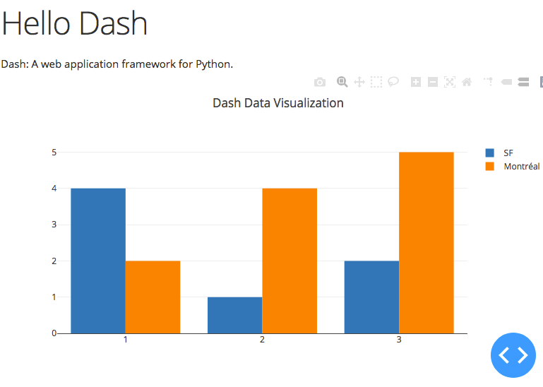
  html.H1(children='Hello Dash'),

  html.Div(children='''
    Dash: A web application framework for Python.
  '''),

  dcc.Graph(
    id='example-graph',
    figure={
      'data': [
        {'x': [1, 2, 3], 'y': [4, 1, 2], 'type': 'bar', 'name': 'SF'},
        {'x': [1, 2, 3], 'y': [2, 4, 5], 'type': 'bar', 'name': u'Montréal'},
      ],
      'layout': {
        'title': 'Dash Data Visualization'
      }
    }
  )
])

if __name__ == '__main__':
  app.run_server(host='0.0.0.0', port=8080, debug=True)

I won’t explain too much of that code here, because this just is the first code example from the Dash manual. But note that I changed the parameters of app.run_server(). You can use any parameter here that the Flask server accepts.

To fire this all up, use first docker-compose build to build the Python image. Then use docker-compose up -d to start both services in the background. To see if they run as ppalnned use docker-compose ps. You should see two services:

Name         Command                         State  Ports
-----------------------------------------------------------------------------
dash_dash    python app.py                   Up     0.0.0.0:80->8080/tcp
dash_pgsql   docker-entrypoint.sh postgres   Up     0.0.0.0:5432->5432/tcp

Now point your browser to http://localhost (or appending whatever port you have used in the docker-compose file) and you should see:

You now can use any editor on your machine to modify the sourcecode in the project directory. Changes will be loaded automatically. If you want to look at the log output of the dash container, use docker-compose logs -f dash and you should see the typical stdout of a Flask application, including the debugger pin, something like:

dash_1 | Running on http://0.0.0.0:8080/
dash_1 | Debugger PIN: 561-251-916
dash_1 | * Serving Flask app "app" (lazy loading)
dash_1 | * Environment: production
dash_1 | WARNING: This is a development server. Do not use it in a production deployment.
dash_1 | Use a production WSGI server instead.
dash_1 | * Debug mode: on
dash_1 | Running on http://0.0.0.0:8080/
dash_1 | Debugger PIN: 231-410-660

Here you will also see when you save a new version of app.py and the web server reloads the app. To stop the environment first use CTRL-c to exit the log tailing and issue a docker-compose down. In an upcoming episode I might show you some more things you cound do with Dash and a database.

Article
0 comment

Graph libraries – D3.js

One of the best known visualization frameworks is D3.js. Written by Mike Bostock, the data visualization superstar about whom Edward Tufte said “that he will become one of the most important people for the future of data visualisation” (according to Wikipedia). And who am I to object to Edward Tufte?

So D3 is in its core an SVG handling library around which several so called layouts for different (actually a lot of) types of diagrams gather. One of them is the so called force-directed graph, which is exactly what we will use here.

How does it look?

This is a real physical simulation (although featuring some shortcuts for reduced calculation time) which means that the arrangement of the nodes when reloading the page is a new one every time and dragging around one node lets the others wobble around. One of the shortcuts is that the repulsive force only is active between nodes connected. So dangling ends can cross edges with the rest of the graph. Nevertheless playing around with the mesh can be fun for some time. The complete source code can be found in the GitHub-Mark-32px GitHub repository

How does it work?

Once again it all starts with including the libraries:

<script src="/graphs/common/jquery-2.1.3.js"></script>
<script src="/graphs/common/d3.js"></script>

The we add some style for nodes and text:

<style>
    .node g text {
        font: 10px sans-serif;
        pointer-events: none;
        text-anchor: middle;
    }
    .node:not(:hover) .nodetext {
        display: none;
    }
    text {
        fill: #000;
        font: 10px sans-serif;
        pointer-events: none;
    }
</style>

Next we define some variables:

var width = 800, height = 500;
var n = 10000, force, svg, drag;

The first line defines width and height of the SVG element, the second line defines n as the number of iterations to be done (I’ll explain later) and the global variables force, svg and drag.

Next we need to define the nodes and edges or links. For the sake of simplicity I’ll do that once again inline. In a real application you would load the dataset in the background:

var nodes = [
    {
        "name": "Node 1",
        "nodeid": 1,
        "nodecolor": "#88cc88",
        "x": 0,
        "y": 0,
    },
...
    {
        "name": "Node 6",
        "nodeid": 6,
        "nodecolor": "#888888",
        "x": 0,
        "y": 0,
    }
];
var links = [
    {
        "source": 0,
        "target": 1,
        "linkcolor": "#888888"
    },
...
    {
        "source": 3,
        "target": 5,
        "linkcolor": "#888888"
    }
];

Then I wrapped up the whole generation and execution of the graph into a function called performGraph():

function performGraph() {
    force = d3.layout.force()
            .charge(-1000)
            .theta(1)
            .linkDistance(170)
            .size([width, height])
            .on("tick", tick);
    drag = force.drag()
            .on("dragstart", dragstart)
            .on("dragend", dragend);
    svg = d3.select("body").append("svg")
            .attr("id", "thissvg")
            .attr("width", width)
            .attr("height", height);
    link = svg.selectAll(".link");
    node = svg.selectAll(".node");
    force.nodes(nodes).links(links);
    force.start();
    for (var i = n; i > 0; --i) {
        force.tick();
    }
    force.stop();
    link = link.data(links)
            .enter()
            .append("g")
            .attr("class", "glink")
            .append("line")
            .style("stroke-width", "3")
            .attr("class", "link")
            .attr("x1", function (d) {
                return d.source.x;
            })
            .attr("y1", function (d) {
                return d.source.y;
            })
            .attr("x2", function (d) {
                return d.target.x;
            })
            .attr("y2", function (d) {
                return d.target.y;
            })
            .attr("stroke", function (d) {
                return d.linkcolor;
            });
    node = node.data(nodes)
            .enter().append("g")
            .attr("class", "node")
            .attr("nodeid", function (d) {
                return d.nodeid
            })
            .attr("transform", function (d) {
                return "translate(" + d.x + "," + d.y + ")";
            });
    node.append("circle")
            .attr("r", "15")
            .attr("fill", function (d) {
                return d.nodecolor;
            })
            //.attr("fill", "#888888")
            .attr("fill-opacity", "1")
            .attr("cx", "0")
            .attr("cy", "0");
    node.append("text")
            .attr("x", 12)
            .attr("dx", "0.5em")
            .attr("dy", "0.5em")
            .attr("class", "nodecaption")
            .attr("display", "inline")
            .text(function (d) {
                return d.name;
            });
    node.call(drag);
}

Lines 2 to 7 set up the force layout engine with some physical parameters, the width and height and an event handler for the ticks. Ticks are D3’s simulation steps. For every tick, a function is called and the positions of the elements are recalculated. We’ll discuss the tick function further down.

Then we define a drag event listener in line 8 to 10 binding its events to two functions called dragstart and dragend. More on those later. Lines 11 to 14 show how to manipulatie the DOM using D3 by adding an SVG element with some attributes to the body.

Lines 15 and 16 handle one of the (for me) most counterintuitive features of D3: we select DOM elements by class that aren’t yet there. Line 17 attaches the nodes and links datasets to the force layout. Line 18 kicks off the physical simulation, line 22 stops it. The for-loop in between counting down from 10000 (the n variable, you remember?) executes 10000 times the force.tick() function. We also could have started the simulation and let it run infinitely but this start-stop handling provides for a steady graph instead of one always wiggling around a bit.

Lines 23 to 44 define, what to do with the links by appending a g (for group) SVG element to the SVG canvas and adding line to the group. Lines 45 to 53 do something similar with the nodes adding a group and a transformation function. In lines 54 to 62 we add a AVG circle element using the nodecolor attribute from the nodes dataset. Lines 63 to 71 finally add the text label to the nodes. Line 72 eventually binds the nodes to the drag event object to allow for the dragging of nodes with a mouse.

Now we need to define all the helper functions bound to event listeners in code above. First the tick() function to do the simulation steps:

function tick() {
    link.attr("x1", function (d) {
        return d.source.x;
    })
    .attr("y1", function (d) {
        return d.source.y;
    })
    .attr("x2", function (d) {
        return d.target.x;
    })
    .attr("y2", function (d) {
        return d.target.y;
    });
    node.attr("transform", function (d) {
        return "translate(" + d.x + "," + d.y + ")";
    });
}

And the dragging functions:

function dragstart(d) {
    force.stop();
}

function dragend(d) {
    force.stop();
}

The last thing to do: kick it to action by calling performGraph():

performGraph();

Why exactly did I put all the code into a function to call it in the end? In a real application you would have some additional GUI elements for example to switch on and of different types of nodes or labels etc. Every time this is done we need to recalculate the graph. Now this can be done with one function call.

Article
1 comment

Graph libraries – Cytoscape.js with Cola.js

Now it’s time for my favourite graph visualization framework. As an introduction I cite from the Cytoscape website:

Cytoscape is an open source software platform for visualizing molecular interaction networks and biological pathways and integrating these networks with annotations, gene expression profiles and other state data.

Cytoscape.js as a side project is a JavaScript library designed to build graph theory related data evaluation and visualization applications on the web. It comes with some layout renderers but is open to other visualization libraries such as Cola.js. Cola is a constraint based layout library with some very interesting features. In this context, we will use it only as a layout engine for the graph.

How does it look?

When playing around with this graph you will probably notice two things:

  1. When dragging around a single node all the other nodes of the graph remain calm and don’t wiggle around like in most physical based layouts.
  2. When reloading this page you will always see the same arrangement of nodes. The graph is stable to reloads.

These two feature result from the way Cola.js renders the graph and are very useful for real world applications. While it’s big fun wobbling and dragging around nodes in a real application you would always like to see the same graph when reloading the same data. And manipulating the arrangement should not affect nodes not touched. The complete source code can be found in the GitHub-Mark-32px GitHub repository.

How does it work?

Once again we start by including the stuff needed. And this are the two libraries and an adaptor to use Cola.js from within Cytoscape.js:

<script src="/graphs/common/cola.js"></script>
<script src="/graphs/common/cytoscape.js"></script>
<script src="/graphs/common/cytoscape-cola.js"></script>

The adaptor can also be found on GitHub.

The HTML body contains a div to render the graph into:

<div id="cy"></div>

The remainder of the index.html file consists of a script:

var elems = [
    {data: {id: '1', name: 'Node 1', nodecolor: '#88cc88'}},
    {data: {id: '2', name: 'Node 2', nodecolor: '#888888'}},
    {data: {id: '3', name: 'Node 3', nodecolor: '#888888'}},
    {data: {id: '4', name: 'Node 4', nodecolor: '#888888'}},
    {data: {id: '5', name: 'Node 5', nodecolor: '#888888'}},
    {data: {id: '6', name: 'Node 6', nodecolor: '#888888'}},
    {
        data: {
            id: '12',
            source: '1',
            target: '2',
            linkcolor: '#888888'
        },
    },
    {
        data: {
            id: '13',
            source: '1',
            target: '3',
            linkcolor: '#888888'
        },
    },
    {
        data: {
            id: '24',
            source: '2',
            target: '4',
            linkcolor: '#ff8888'
        },
    },
    {
        data: {
            id: '25',
            source: '2',
            target: '5',
            linkcolor: '#ff8888'
        },
    },
    {
        data: {
            id: '45',
            source: '4',
            target: '5',
            linkcolor: '#ff8888'
        }
    },
    {
        data: {
            id: '46',
            source: '4',
            target: '6',
            linkcolor: '#888888'
        }
    }];
var cy = cytoscape({
    container: document.getElementById('cy'),
    elements: elems,
    style: cytoscape.stylesheet()
            .selector('node').style({
                'background-color': 'data(nodecolor)',
                label: 'data(name)',
                width: 25,
                height: 25
            })
            .selector('edge').style({
                'line-color': 'data(linkcolor)',
                width: 3
            })
});
cy.layout({name: 'cola', padding: 10});

Lines 2 to 7 define the nodes with their name/caption and colour. Lines 8 to 54 define the edges in a similar way. Lines 56 to 70 define the Cytoscape container and attach dynamic properties to the nodes and edges. Line 71 finally kicks off the layout rendering. Note: up to that last line we specified exactly no rendering or geometry information! By changing the name of the renderer from cola  to one of the built-ins (circle  or cose  are fun to play with!) you can get a completely different outout.

As a last remark I strongly recommend to have a look at the graph theoretical and practical routines and algorithms the Cytoscape.js library has to offer.

Article
0 comment

Graph libraries – Arbor.js

Arbor.js is written by Christian Swineheart from Samizdat Drafting Co. The documentation is concise even though the main page navigation as animated tree layout always drives me crazy :) The example I present here only depends on arbor.js and jQuery. Graph definition is for shortness and clarity done by calls to addNode  and addEdge  methods of the ParticleSystem renderer.

How does it look?

As you can see, the physical simulation is much more fluid and undamped than with Alchemy.js. I’m pretty much shure this can be changed to some degree with a different initialization of the particle system as described in the reference documentation. Once again, the complete source code, in this case consisting only of an index.html file, can be found in the GitHub-Mark-32px GitHub repository.

How does it work?

Once again in the header we start by loading the stuff needed:

<script src="/graphs/common/jquery-2.1.3.js"></script>
<script src="/graphs/common/arbor.js"></script>
<script src="/graphs/common/arbor-tween.js"></script>

arbor-tween.js is not really needed for this example as it allows gradual transitions in the data object of nodes and edges. Arbor.js by default renders its graph in a HTML5 canvas, in the body we need to define this:

<canvas id="viewport" width="800" height="500"></canvas>

The remainder of the file consists of a function defining and binding the renderer object to the canvas and constructing the graph:

(function ($) {
        var Renderer = function (canvas) {
                var canvas = $(canvas).get(0);
                var ctx = canvas.getContext("2d");
                var particleSystem;
                var that = {
                        init: function (system) {
                                particleSystem = system;
                                particleSystem.screenSize(canvas.width, canvas.height);
                                particleSystem.screenPadding(100);
                                that.initMouseHandling()
                        },
                        redraw: function () {
                                ctx.fillStyle = "white";
                                ctx.fillRect(0, 0, canvas.width, canvas.height);
                                particleSystem.eachEdge(function (edge, pt1, pt2) {
                                        ctx.strokeStyle = edge.data.linkcolor;
                                        ctx.lineWidth = 3;
                                        ctx.beginPath();
                                        ctx.moveTo(pt1.x, pt1.y);
                                        ctx.lineTo(pt2.x, pt2.y);
                                        ctx.stroke();
                                });
                                particleSystem.eachNode(function (node, pt) {
                                        ctx.beginPath();
                                        ctx.arc(pt.x, pt.y, 15, 0, 2 * Math.PI);
                                        ctx.fillStyle = node.data.nodecolor;
                                        ctx.fill();
                                        ctx.font = "18px Arial";
                                        ctx.fillStyle = "#000000";
                                        ctx.fillText(node.data.name, pt.x + 20, pt.y + 5);
                                });
                        },
                        initMouseHandling: function () {
                                var dragged = null;
                                var handler = {
                                        clicked: function (e) {
                                                var pos = $(canvas).offset();
                                                _mouseP = arbor.Point(e.pageX - pos.left, e.pageY - pos.top);
                                                dragged = particleSystem.nearest(_mouseP);
                                                if (dragged && dragged.node !== null) {
                                                        dragged.node.fixed = true;
                                                }
                                                $(canvas).bind('mousemove', handler.dragged);
                                                $(window).bind('mouseup', handler.dropped);
                                                return false;
                                        },
                                        dragged: function (e) {
                                                var pos = $(canvas).offset();
                                                var s = arbor.Point(e.pageX - pos.left, e.pageY - pos.top);
                                                if (dragged && dragged.node !== null) {
                                                        var p = particleSystem.fromScreen(s);
                                                        dragged.node.p = p
                                                }
                                                return false;
                                        },
                                        dropped: function (e) {
                                                if (dragged === null || dragged.node === undefined) return;
                                                if (dragged.node !== null) dragged.node.fixed = false;
                                                dragged.node.tempMass = 1000;
                                                dragged = null;
                                                $(canvas).unbind('mousemove', handler.dragged);
                                                $(window).unbind('mouseup', handler.dropped);
                                                _mouseP = null;
                                                return false;
                                        }
                                };
                                $(canvas).mousedown(handler.clicked);
                        }
                }
                return that;
        }
        $(document).ready(function () {
                var sys = arbor.ParticleSystem(700, 700, 0.5);
                sys.renderer = Renderer("#viewport");
                sys.addNode('Node 1', {name: "Node 1", nodecolor: "#88cc88"});
                sys.addNode('Node 2', {name: "Node 2", nodecolor: "#888888"});
                sys.addNode('Node 3', {name: "Node 3", nodecolor: "#888888"});
                sys.addNode('Node 4', {name: "Node 4", nodecolor: "#888888"});
                sys.addNode('Node 5', {name: "Node 5", nodecolor: "#888888"});
                sys.addNode('Node 6', {name: "Node 6", nodecolor: "#888888"});
                sys.addEdge('Node 1', 'Node 3', {linkcolor: "#888888"});
                sys.addEdge('Node 1', 'Node 2', {linkcolor: "#888888"});
                sys.addEdge('Node 2', 'Node 5', {linkcolor: "#ff8888"});
                sys.addEdge('Node 2', 'Node 4', {linkcolor: "#ff8888"});
                sys.addEdge('Node 4', 'Node 5', {linkcolor: "#ff8888"});
                sys.addEdge('Node 5', 'Node 6', {linkcolor: "#888888"});
        })
})(this.jQuery);

Lines 2 to 73 define the Renderer, in detail:

  • get the HTML5 canvas (line 3)
  • grab its 2D context (line 4)
  • an init function for the particle system (lines 7 to 12)
  • a redraw function actually drawing the graph (lines 13 to 33) by iterating over all nodes and edges
  • defining a pretty basic mouse handling (lines 34 to 69)

In line 75 we get a particle system, set the rendering to the canvas in line 76 and define nodes (lines 76 to 81) and edges (lines 82 to 87). That’s pretty much all.

Article
3 comments

Graph libraries – Alchemy.js

Alchemy.js is a library developed by graphAlchemist (site defunct). The documentation could be better and more detailed but it works. Like many other libraries it leverages other libraries to do “the basic stuff”. In this case it is it depends on:

Alchemy uses GraphJSON (similar to GeoJSON) as input format, which is quite nice but undocumented since the website graphjson.io doesn’t exist any more. Looks as if support for it ceded with the graphAlchemist web site …

How does it look?

Like all demos I’ll show it’s a fully functional mini demo, so you can drag the nodes around. I’ll present excerpts of the code to explain. The complete code can be found in a GitHub-Mark-32px GitHub repository.

How does it work?

Our example consists of an index.html file, a GraphJSON data file and the library stuff. In the index.html we first load the stuff needed:

<link rel="stylesheet" href="/graphs/common/alchemy/alchemy.css"/>
<script src="/graphs/common/jquery-2.1.3.js"></script>
<script src="/graphs/common/d3.js"></script>
<script src="/graphs/common/lodash.js"></script>

The body contains a div to put the graph in and the include for the base library itself:

<div class="alchemy" id="alchemy"></div>
<script src="/graphs/common/alchemy/alchemy.js"></script>

Finally there’s the code producing the graph:

var config = {
    dataSource: '/graphs/alchemy/data/network.json',
    graphWidth: function() {return 800},
    graphHeight: function() {return 500},
    backgroundColor: "#ffffff",
    nodeCaptionsOnByDefault: true,
    caption: function(node){
        return node.caption;
    },
    nodeTypes: {
        "role": ["greyone", "greenone"]
    },
    edgeTypes: {
        "caption": ["greyone", "redone"]
    },
    nodeStyle: {
        "greyone": {
            color: "#888888",
            borderWidth: 0,
            radius: 15
        },
        "greenone": {
            color: "#88cc88",
            borderWidth: 0,
            radius: 15
        }
    },
    edgeStyle: {
        "greyone": {
            color: "#888888",
            width: 3
        },
        "redone": {
            color: "#ff8888",
            width: 3
        }
    }
};
alchemy = new Alchemy(config)

As you can see, nearly everything is done in a configuration object. Line 2 defines the source of the GraphJSON file, lines 3 & 4 set the dimensions of the SVG element. The setting of nodeCaptionsOnByDefault  in line 6 switches on the display of the node titles. Otherwise they would only show up when hovering with the mouse. Lines 7 to 9 define a callback function defining what to display as a caption / title. Lines 10 to 15 define valid values for grouping edges and nodes. Nodes are grouped by the role attribute, edges by caption. Lines 16 to 37 define how these groups of edges and nodes should be formatted. There are other, more direct ways to style a graph in Alchemy.js but I wanted to show the (for me) most elegant way. Finally line 39 kicks off the rendering of the graph with the given configuration.

Article
0 comment

Graph libraries – Introduction

This post starts a small series of articles, that will present some JavaScript graph plotting libraries and show how to draw more or less the same simple demo graph with these different libs.

What is a graph?

Graph theory is a mathematical discipline that studies networks of nodes and links or edges connecting them. Graphs are useful for many applications: social media networks, streets connecting cities, transfers connecting bank accounts or networks of people, addresses, bank accounts and cars connected via insurance claims and events. We’ll deal with some of those applications later on when discussing the application of network and graph paradigms to visualizing fraudulent actions.

Which libraries have I examined?

The internet is full, I mean literally FULL of libraries to display networked graphs. I had to choose some and discard others. First I decided to neglect commercial libraries that don’t have an open source edition. Then I stopped evaluating libs when I recognized that the documentation is too poor or functionality too limited to further investigate. So here is the list in alphabetical order:

Libraries I didn’t evaluate due to licensing constraints:

Libraries I gave up on:

  • Dracula Graph Library (Graph Dracula … you understand … haha)
    Needs a raphael.js renderer to display custom node shapes. Too much fuzz for a very short test.
  • sigma.js
    Poorly documented. Didn’t succeed to build a test candidate in short (!) time.

How did I test?

networkI always used the same test network. It consists of 6 nodes and 6 edges. Some edges are red and one node is green. The nodes are labelled “Node 1” to “Node 6”. Colouring and labelling is used to test how easy it is to insert some basic customization into the layout.

On the right side you can see a hand drawn (well not really handdrawn) picture of the demo network. The examples I present are fully functional, not screen shots and I will briefly go through the source code.

Update

The first part for Alchemy.js can be found here.

The second post on Arbor.js is here.

The third part with Cytoscape.js and Cola.js is here.

The fourth part with D3 is here.

Article
0 comment

Separating structure and semantics

There is a great and simple rule, known as “Micha’s Golden Rule”, which goes back to Micha Gorelick (@mynameisfiber). It states:

Do not store data in the keys of a JSON blob.

This means, that instead of writing a JSON dataset holding people and their gaming scores like this:

{
  "Volker": 100,
  "John": 300
}

you should use something like:

[
  {
    "name": "Volker",
    "score": 100
  },
  {
    "name": "John",
    "score": 300
  }
]

First of all, it is good practice, to separate data and its meaning. Second it simplifies software development. And here is why:

One reason is, that in the first form you have no idea, what exactly the number associated with the name means. And when accessing the data you need to know the keys. But the keys are part of the data. So you first have to parse the whole file, separate the keys and iterate over them. In the second case you can iterate over a set of completely identical structured data sets and fetch names and scores.

This rule not only holds true for JSON but for any structured data like XML or yaml. Consider the following modified XML example from the SimpleXML section of the PHP manual:


  PHP: Behind the Parser
  Rasmus Lerdorf
  1
 

In PHP you would access the director in this way:

movie[0]->director;
?>

Now if you would like to use the directors name as a key to get the number of oscars he won, it would look like:


  PHP: Behind the Parser
  1
 

This is perfectly valid but stupid XML. And to access the data you need to know the name of the director:

movie[0]->RasmusLerdorf;
?>

Doesn’t make too much sense, hm? One additional drawback I didn’t mention but that you nevertheless saw: the keys of a data structure language often are subject to several limitaions. In XML element names e.g. there can’t be spaces. So you have to work around that e.g. by camelcasing the name. To get the name back in readable form, you would have to parse it and insert spaces at the correct positions. Which can be impossible with human names, since there are camelcased names like “DeLorean”.

Considering this rule is not always obvious but can save you a lot of nerves. Take care!