Article
0 comment

Graph libraries – D3.js

One of the best known visualization frameworks is D3.js. Written by Mike Bostock, the data visualization superstar about whom Edward Tufte said “that he will become one of the most important people for the future of data visualisation” (according to Wikipedia). And who am I to object to Edward Tufte?

So D3 is in its core an SVG handling library around which several so called layouts for different (actually a lot of) types of diagrams gather. One of them is the so called force-directed graph, which is exactly what we will use here.
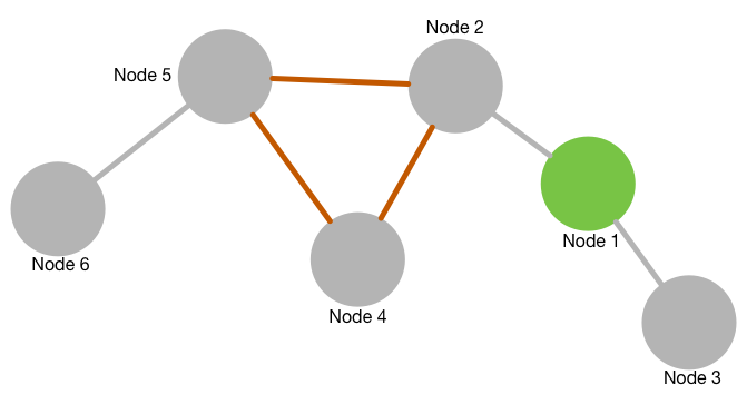
How does it look?

This is a real physical simulation (although featuring some shortcuts for reduced calculation time) which means that the arrangement of the nodes when reloading the page is a new one every time and dragging around one node lets the others wobble around. One of the shortcuts is that the repulsive force only is active between nodes connected. So dangling ends can cross edges with the rest of the graph. Nevertheless playing around with the mesh can be fun for some time. The complete source code can be found in the GitHub-Mark-32px GitHub repository

How does it work?

Once again it all starts with including the libraries:

<script src="/graphs/common/jquery-2.1.3.js"></script>
<script src="/graphs/common/d3.js"></script>

The we add some style for nodes and text:

<style>
    .node g text {
        font: 10px sans-serif;
        pointer-events: none;
        text-anchor: middle;
    }
    .node:not(:hover) .nodetext {
        display: none;
    }
    text {
        fill: #000;
        font: 10px sans-serif;
        pointer-events: none;
    }
</style>

Next we define some variables:

var width = 800, height = 500;
var n = 10000, force, svg, drag;

The first line defines width and height of the SVG element, the second line defines n as the number of iterations to be done (I’ll explain later) and the global variables force, svg and drag.

Next we need to define the nodes and edges or links. For the sake of simplicity I’ll do that once again inline. In a real application you would load the dataset in the background:

var nodes = [
    {
        "name": "Node 1",
        "nodeid": 1,
        "nodecolor": "#88cc88",
        "x": 0,
        "y": 0,
    },
...
    {
        "name": "Node 6",
        "nodeid": 6,
        "nodecolor": "#888888",
        "x": 0,
        "y": 0,
    }
];
var links = [
    {
        "source": 0,
        "target": 1,
        "linkcolor": "#888888"
    },
...
    {
        "source": 3,
        "target": 5,
        "linkcolor": "#888888"
    }
];

Then I wrapped up the whole generation and execution of the graph into a function called performGraph():

function performGraph() {
    force = d3.layout.force()
            .charge(-1000)
            .theta(1)
            .linkDistance(170)
            .size([width, height])
            .on("tick", tick);
    drag = force.drag()
            .on("dragstart", dragstart)
            .on("dragend", dragend);
    svg = d3.select("body").append("svg")
            .attr("id", "thissvg")
            .attr("width", width)
            .attr("height", height);
    link = svg.selectAll(".link");
    node = svg.selectAll(".node");
    force.nodes(nodes).links(links);
    force.start();
    for (var i = n; i > 0; --i) {
        force.tick();
    }
    force.stop();
    link = link.data(links)
            .enter()
            .append("g")
            .attr("class", "glink")
            .append("line")
            .style("stroke-width", "3")
            .attr("class", "link")
            .attr("x1", function (d) {
                return d.source.x;
            })
            .attr("y1", function (d) {
                return d.source.y;
            })
            .attr("x2", function (d) {
                return d.target.x;
            })
            .attr("y2", function (d) {
                return d.target.y;
            })
            .attr("stroke", function (d) {
                return d.linkcolor;
            });
    node = node.data(nodes)
            .enter().append("g")
            .attr("class", "node")
            .attr("nodeid", function (d) {
                return d.nodeid
            })
            .attr("transform", function (d) {
                return "translate(" + d.x + "," + d.y + ")";
            });
    node.append("circle")
            .attr("r", "15")
            .attr("fill", function (d) {
                return d.nodecolor;
            })
            //.attr("fill", "#888888")
            .attr("fill-opacity", "1")
            .attr("cx", "0")
            .attr("cy", "0");
    node.append("text")
            .attr("x", 12)
            .attr("dx", "0.5em")
            .attr("dy", "0.5em")
            .attr("class", "nodecaption")
            .attr("display", "inline")
            .text(function (d) {
                return d.name;
            });
    node.call(drag);
}

Lines 2 to 7 set up the force layout engine with some physical parameters, the width and height and an event handler for the ticks. Ticks are D3’s simulation steps. For every tick, a function is called and the positions of the elements are recalculated. We’ll discuss the tick function further down.

Then we define a drag event listener in line 8 to 10 binding its events to two functions called dragstart and dragend. More on those later. Lines 11 to 14 show how to manipulatie the DOM using D3 by adding an SVG element with some attributes to the body.

Lines 15 and 16 handle one of the (for me) most counterintuitive features of D3: we select DOM elements by class that aren’t yet there. Line 17 attaches the nodes and links datasets to the force layout. Line 18 kicks off the physical simulation, line 22 stops it. The for-loop in between counting down from 10000 (the n variable, you remember?) executes 10000 times the force.tick() function. We also could have started the simulation and let it run infinitely but this start-stop handling provides for a steady graph instead of one always wiggling around a bit.

Lines 23 to 44 define, what to do with the links by appending a g (for group) SVG element to the SVG canvas and adding line to the group. Lines 45 to 53 do something similar with the nodes adding a group and a transformation function. In lines 54 to 62 we add a AVG circle element using the nodecolor attribute from the nodes dataset. Lines 63 to 71 finally add the text label to the nodes. Line 72 eventually binds the nodes to the drag event object to allow for the dragging of nodes with a mouse.

Now we need to define all the helper functions bound to event listeners in code above. First the tick() function to do the simulation steps:

function tick() {
    link.attr("x1", function (d) {
        return d.source.x;
    })
    .attr("y1", function (d) {
        return d.source.y;
    })
    .attr("x2", function (d) {
        return d.target.x;
    })
    .attr("y2", function (d) {
        return d.target.y;
    });
    node.attr("transform", function (d) {
        return "translate(" + d.x + "," + d.y + ")";
    });
}

And the dragging functions:

function dragstart(d) {
    force.stop();
}

function dragend(d) {
    force.stop();
}

The last thing to do: kick it to action by calling performGraph():

performGraph();

Why exactly did I put all the code into a function to call it in the end? In a real application you would have some additional GUI elements for example to switch on and of different types of nodes or labels etc. Every time this is done we need to recalculate the graph. Now this can be done with one function call.

Article
0 comment

Innovation means breaking the rules

6264574707_47f374a312_oToday I paged through a book by Martin Gaedt, called “Rock your idea”. Despite the  english title the book is written in German. One of the first and central ideas presented there was:

Innovation means to break the rules.

I’ve been scientific and innovation enabler for several projects and companies now and this is nearly all you need to know about injecting new ideas or technology into companies.

If you want to work out a totally different and optimal solution for a given  problem or even want to create a new area of business, you have to break the rules.

  • The rules defining what is possible. Maybe someone just invented the technology needed to build your idea. You might at the moment not know that.
  • The rules what we think customers need or want. Ever heard that argument “None of our customers asked for that! Why should we build that?”?.
  • The rules of the existing business. Ever heard that your idea doesn’t fit into the portfolio of the company? WHAT THE HECK? The portfolio is where the money is, for God’s sake!
  • And sometimes even the rules of hierarchy. Having an innovator working ‘at a short leash’ often means preventing innovation. Sometimes managerial control is the worst you can do to harm your company.

So to reformulate the negative arguments to positive actionable items:

  • When having a new idea, don’t instantly think about existing technology to build it. When you need it, there will be a solution. There always was one when I needed it. Finding technical solutions is the job of people like me.
  • When you don’t know if a customers will buy into your idea, TALK TO THEM. Sometimes you will get a piloting customer aboard for an idea that is nothing more than that: an idea. Sometimes you will have to invest a small amount of money and time into a prototype or mockup to win a customers interest.
  • If you only look for ideas fitting into an existing portfolio, I’m sorry to tell you, that your company will not have any chances to survive a future disruptive change in its very own field of business. There will be someone else having a similar idea and with no reluctance to realize it, portfolio or not.
  • If you have people working for you on innovative ideas, trust them. At least a bit further than you feel comfortable with. Micromanaging people is a great way to let them look for another company that offers a broader field of work. If you expect your researchers to follow working instructions to the point you’re exactly missing the point.
Article
1 comment

Graph libraries – Cytoscape.js with Cola.js

Now it’s time for my favourite graph visualization framework. As an introduction I cite from the Cytoscape website:

Cytoscape is an open source software platform for visualizing molecular interaction networks and biological pathways and integrating these networks with annotations, gene expression profiles and other state data.

Cytoscape.js as a side project is a JavaScript library designed to build graph theory related data evaluation and visualization applications on the web. It comes with some layout renderers but is open to other visualization libraries such as Cola.js. Cola is a constraint based layout library with some very interesting features. In this context, we will use it only as a layout engine for the graph.

How does it look?

When playing around with this graph you will probably notice two things:

  1. When dragging around a single node all the other nodes of the graph remain calm and don’t wiggle around like in most physical based layouts.
  2. When reloading this page you will always see the same arrangement of nodes. The graph is stable to reloads.

These two feature result from the way Cola.js renders the graph and are very useful for real world applications. While it’s big fun wobbling and dragging around nodes in a real application you would always like to see the same graph when reloading the same data. And manipulating the arrangement should not affect nodes not touched. The complete source code can be found in the GitHub-Mark-32px GitHub repository.

How does it work?

Once again we start by including the stuff needed. And this are the two libraries and an adaptor to use Cola.js from within Cytoscape.js:

<script src="/graphs/common/cola.js"></script>
<script src="/graphs/common/cytoscape.js"></script>
<script src="/graphs/common/cytoscape-cola.js"></script>

The adaptor can also be found on GitHub.

The HTML body contains a div to render the graph into:

<div id="cy"></div>

The remainder of the index.html file consists of a script:

var elems = [
    {data: {id: '1', name: 'Node 1', nodecolor: '#88cc88'}},
    {data: {id: '2', name: 'Node 2', nodecolor: '#888888'}},
    {data: {id: '3', name: 'Node 3', nodecolor: '#888888'}},
    {data: {id: '4', name: 'Node 4', nodecolor: '#888888'}},
    {data: {id: '5', name: 'Node 5', nodecolor: '#888888'}},
    {data: {id: '6', name: 'Node 6', nodecolor: '#888888'}},
    {
        data: {
            id: '12',
            source: '1',
            target: '2',
            linkcolor: '#888888'
        },
    },
    {
        data: {
            id: '13',
            source: '1',
            target: '3',
            linkcolor: '#888888'
        },
    },
    {
        data: {
            id: '24',
            source: '2',
            target: '4',
            linkcolor: '#ff8888'
        },
    },
    {
        data: {
            id: '25',
            source: '2',
            target: '5',
            linkcolor: '#ff8888'
        },
    },
    {
        data: {
            id: '45',
            source: '4',
            target: '5',
            linkcolor: '#ff8888'
        }
    },
    {
        data: {
            id: '46',
            source: '4',
            target: '6',
            linkcolor: '#888888'
        }
    }];
var cy = cytoscape({
    container: document.getElementById('cy'),
    elements: elems,
    style: cytoscape.stylesheet()
            .selector('node').style({
                'background-color': 'data(nodecolor)',
                label: 'data(name)',
                width: 25,
                height: 25
            })
            .selector('edge').style({
                'line-color': 'data(linkcolor)',
                width: 3
            })
});
cy.layout({name: 'cola', padding: 10});

Lines 2 to 7 define the nodes with their name/caption and colour. Lines 8 to 54 define the edges in a similar way. Lines 56 to 70 define the Cytoscape container and attach dynamic properties to the nodes and edges. Line 71 finally kicks off the layout rendering. Note: up to that last line we specified exactly no rendering or geometry information! By changing the name of the renderer from cola  to one of the built-ins (circle  or cose  are fun to play with!) you can get a completely different outout.

As a last remark I strongly recommend to have a look at the graph theoretical and practical routines and algorithms the Cytoscape.js library has to offer.

Article
0 comment

Graph libraries – Arbor.js

Arbor.js is written by Christian Swineheart from Samizdat Drafting Co. The documentation is concise even though the main page navigation as animated tree layout always drives me crazy :) The example I present here only depends on arbor.js and jQuery. Graph definition is for shortness and clarity done by calls to addNode  and addEdge  methods of the ParticleSystem renderer.

How does it look?

As you can see, the physical simulation is much more fluid and undamped than with Alchemy.js. I’m pretty much shure this can be changed to some degree with a different initialization of the particle system as described in the reference documentation. Once again, the complete source code, in this case consisting only of an index.html file, can be found in the GitHub-Mark-32px GitHub repository.

How does it work?

Once again in the header we start by loading the stuff needed:

<script src="/graphs/common/jquery-2.1.3.js"></script>
<script src="/graphs/common/arbor.js"></script>
<script src="/graphs/common/arbor-tween.js"></script>

arbor-tween.js is not really needed for this example as it allows gradual transitions in the data object of nodes and edges. Arbor.js by default renders its graph in a HTML5 canvas, in the body we need to define this:

<canvas id="viewport" width="800" height="500"></canvas>

The remainder of the file consists of a function defining and binding the renderer object to the canvas and constructing the graph:

(function ($) {
        var Renderer = function (canvas) {
                var canvas = $(canvas).get(0);
                var ctx = canvas.getContext("2d");
                var particleSystem;
                var that = {
                        init: function (system) {
                                particleSystem = system;
                                particleSystem.screenSize(canvas.width, canvas.height);
                                particleSystem.screenPadding(100);
                                that.initMouseHandling()
                        },
                        redraw: function () {
                                ctx.fillStyle = "white";
                                ctx.fillRect(0, 0, canvas.width, canvas.height);
                                particleSystem.eachEdge(function (edge, pt1, pt2) {
                                        ctx.strokeStyle = edge.data.linkcolor;
                                        ctx.lineWidth = 3;
                                        ctx.beginPath();
                                        ctx.moveTo(pt1.x, pt1.y);
                                        ctx.lineTo(pt2.x, pt2.y);
                                        ctx.stroke();
                                });
                                particleSystem.eachNode(function (node, pt) {
                                        ctx.beginPath();
                                        ctx.arc(pt.x, pt.y, 15, 0, 2 * Math.PI);
                                        ctx.fillStyle = node.data.nodecolor;
                                        ctx.fill();
                                        ctx.font = "18px Arial";
                                        ctx.fillStyle = "#000000";
                                        ctx.fillText(node.data.name, pt.x + 20, pt.y + 5);
                                });
                        },
                        initMouseHandling: function () {
                                var dragged = null;
                                var handler = {
                                        clicked: function (e) {
                                                var pos = $(canvas).offset();
                                                _mouseP = arbor.Point(e.pageX - pos.left, e.pageY - pos.top);
                                                dragged = particleSystem.nearest(_mouseP);
                                                if (dragged && dragged.node !== null) {
                                                        dragged.node.fixed = true;
                                                }
                                                $(canvas).bind('mousemove', handler.dragged);
                                                $(window).bind('mouseup', handler.dropped);
                                                return false;
                                        },
                                        dragged: function (e) {
                                                var pos = $(canvas).offset();
                                                var s = arbor.Point(e.pageX - pos.left, e.pageY - pos.top);
                                                if (dragged && dragged.node !== null) {
                                                        var p = particleSystem.fromScreen(s);
                                                        dragged.node.p = p
                                                }
                                                return false;
                                        },
                                        dropped: function (e) {
                                                if (dragged === null || dragged.node === undefined) return;
                                                if (dragged.node !== null) dragged.node.fixed = false;
                                                dragged.node.tempMass = 1000;
                                                dragged = null;
                                                $(canvas).unbind('mousemove', handler.dragged);
                                                $(window).unbind('mouseup', handler.dropped);
                                                _mouseP = null;
                                                return false;
                                        }
                                };
                                $(canvas).mousedown(handler.clicked);
                        }
                }
                return that;
        }
        $(document).ready(function () {
                var sys = arbor.ParticleSystem(700, 700, 0.5);
                sys.renderer = Renderer("#viewport");
                sys.addNode('Node 1', {name: "Node 1", nodecolor: "#88cc88"});
                sys.addNode('Node 2', {name: "Node 2", nodecolor: "#888888"});
                sys.addNode('Node 3', {name: "Node 3", nodecolor: "#888888"});
                sys.addNode('Node 4', {name: "Node 4", nodecolor: "#888888"});
                sys.addNode('Node 5', {name: "Node 5", nodecolor: "#888888"});
                sys.addNode('Node 6', {name: "Node 6", nodecolor: "#888888"});
                sys.addEdge('Node 1', 'Node 3', {linkcolor: "#888888"});
                sys.addEdge('Node 1', 'Node 2', {linkcolor: "#888888"});
                sys.addEdge('Node 2', 'Node 5', {linkcolor: "#ff8888"});
                sys.addEdge('Node 2', 'Node 4', {linkcolor: "#ff8888"});
                sys.addEdge('Node 4', 'Node 5', {linkcolor: "#ff8888"});
                sys.addEdge('Node 5', 'Node 6', {linkcolor: "#888888"});
        })
})(this.jQuery);

Lines 2 to 73 define the Renderer, in detail:

  • get the HTML5 canvas (line 3)
  • grab its 2D context (line 4)
  • an init function for the particle system (lines 7 to 12)
  • a redraw function actually drawing the graph (lines 13 to 33) by iterating over all nodes and edges
  • defining a pretty basic mouse handling (lines 34 to 69)

In line 75 we get a particle system, set the rendering to the canvas in line 76 and define nodes (lines 76 to 81) and edges (lines 82 to 87). That’s pretty much all.

Article
3 comments

Graph libraries – Alchemy.js

Alchemy.js is a library developed by graphAlchemist (site defunct). The documentation could be better and more detailed but it works. Like many other libraries it leverages other libraries to do “the basic stuff”. In this case it is it depends on:

Alchemy uses GraphJSON (similar to GeoJSON) as input format, which is quite nice but undocumented since the website graphjson.io doesn’t exist any more. Looks as if support for it ceded with the graphAlchemist web site …

How does it look?

Like all demos I’ll show it’s a fully functional mini demo, so you can drag the nodes around. I’ll present excerpts of the code to explain. The complete code can be found in a GitHub-Mark-32px GitHub repository.

How does it work?

Our example consists of an index.html file, a GraphJSON data file and the library stuff. In the index.html we first load the stuff needed:

<link rel="stylesheet" href="/graphs/common/alchemy/alchemy.css"/>
<script src="/graphs/common/jquery-2.1.3.js"></script>
<script src="/graphs/common/d3.js"></script>
<script src="/graphs/common/lodash.js"></script>

The body contains a div to put the graph in and the include for the base library itself:

<div class="alchemy" id="alchemy"></div>
<script src="/graphs/common/alchemy/alchemy.js"></script>

Finally there’s the code producing the graph:

var config = {
    dataSource: '/graphs/alchemy/data/network.json',
    graphWidth: function() {return 800},
    graphHeight: function() {return 500},
    backgroundColor: "#ffffff",
    nodeCaptionsOnByDefault: true,
    caption: function(node){
        return node.caption;
    },
    nodeTypes: {
        "role": ["greyone", "greenone"]
    },
    edgeTypes: {
        "caption": ["greyone", "redone"]
    },
    nodeStyle: {
        "greyone": {
            color: "#888888",
            borderWidth: 0,
            radius: 15
        },
        "greenone": {
            color: "#88cc88",
            borderWidth: 0,
            radius: 15
        }
    },
    edgeStyle: {
        "greyone": {
            color: "#888888",
            width: 3
        },
        "redone": {
            color: "#ff8888",
            width: 3
        }
    }
};
alchemy = new Alchemy(config)

As you can see, nearly everything is done in a configuration object. Line 2 defines the source of the GraphJSON file, lines 3 & 4 set the dimensions of the SVG element. The setting of nodeCaptionsOnByDefault  in line 6 switches on the display of the node titles. Otherwise they would only show up when hovering with the mouse. Lines 7 to 9 define a callback function defining what to display as a caption / title. Lines 10 to 15 define valid values for grouping edges and nodes. Nodes are grouped by the role attribute, edges by caption. Lines 16 to 37 define how these groups of edges and nodes should be formatted. There are other, more direct ways to style a graph in Alchemy.js but I wanted to show the (for me) most elegant way. Finally line 39 kicks off the rendering of the graph with the given configuration.

Article
0 comment

Graph libraries – Introduction

This post starts a small series of articles, that will present some JavaScript graph plotting libraries and show how to draw more or less the same simple demo graph with these different libs.

What is a graph?

Graph theory is a mathematical discipline that studies networks of nodes and links or edges connecting them. Graphs are useful for many applications: social media networks, streets connecting cities, transfers connecting bank accounts or networks of people, addresses, bank accounts and cars connected via insurance claims and events. We’ll deal with some of those applications later on when discussing the application of network and graph paradigms to visualizing fraudulent actions.

Which libraries have I examined?

The internet is full, I mean literally FULL of libraries to display networked graphs. I had to choose some and discard others. First I decided to neglect commercial libraries that don’t have an open source edition. Then I stopped evaluating libs when I recognized that the documentation is too poor or functionality too limited to further investigate. So here is the list in alphabetical order:

Libraries I didn’t evaluate due to licensing constraints:

Libraries I gave up on:

  • Dracula Graph Library (Graph Dracula … you understand … haha)
    Needs a raphael.js renderer to display custom node shapes. Too much fuzz for a very short test.
  • sigma.js
    Poorly documented. Didn’t succeed to build a test candidate in short (!) time.

How did I test?

networkI always used the same test network. It consists of 6 nodes and 6 edges. Some edges are red and one node is green. The nodes are labelled “Node 1” to “Node 6”. Colouring and labelling is used to test how easy it is to insert some basic customization into the layout.

On the right side you can see a hand drawn (well not really handdrawn) picture of the demo network. The examples I present are fully functional, not screen shots and I will briefly go through the source code.

Update

The first part for Alchemy.js can be found here.

The second post on Arbor.js is here.

The third part with Cytoscape.js and Cola.js is here.

The fourth part with D3 is here.